Product Analytics Queries Without Database Meltdown

I've personally watched this journey unfold — what starts as shipping a simple dashboard can eventually lead to temporary patches, complexity creep, and full rearchitectures just to avoid killing the transactional database. This'll walk you through the journey I've seen a team take many years ago at a fast-scaling startup and help you short-circuit this cycle, saving months of discovery pain along the way.
Meltdown
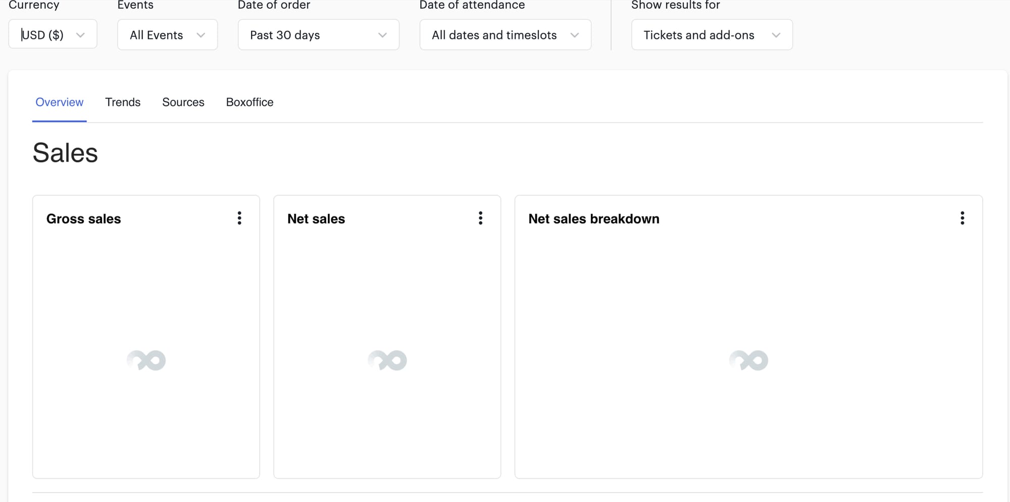
One of our biggest international customers launched a flash sale that drove 50x their normal transaction volume. At 3 AM, our on-call was paged and Slack lit up with alerts. "DATABASE CPU: CRITICAL." "API LATENCY: CRITICAL." "CHECKOUT FAILURE RATE: CRITICAL.". This customer eventually churned due to the lost revenue from the incident. The culprit? Constant refreshing of their dashboard to track sale success.
Let’s take a closer look at the query:
SELECT
  date_trunc('month', purchase_date) as month,
  customer_region,
  AVG(customer_age) as avg_age,
  SUM(purchase_amount) as total_revenue,
  COUNT(DISTINCT customer_id) as unique_customers
FROM purchases
JOIN customers ON purchases.customer_id = customers.id
WHERE purchase_date > NOW() - INTERVAL '12 months'
GROUP BY date_trunc('month', purchase_date), customer_region
ORDER BY month, total_revenue DESC;
When this query executes in a transactional database, several resource-intensive operations occur:
- Full table scan: Without proper indexes, the database reads every row in both tables to find matching records.
- Join operation: The database builds an in-memory hash table for the join, which can consume significant RAM when joining large tables.
- Grouping operation: Another in-memory hash table gets built to track each unique group (month + region).
- Distinct counting: The
COUNT(DISTINCT customer_id)requires tracking all unique customer IDs seen so far, adding more memory pressure. - Sorting: Finally, the results get sorted by month and revenue, potentially needing disk if the result set is large enough.
In transactional databases like PostgreSQL, Multiversion concurrency control (MVCC) avoids locking by letting each query see a consistent snapshot of the data. This works by checking the visibility of each row version at read time. But for large analytical queries—especially those that scan millions of rows and compute aggregates—these per-row checks can spike CPU usage. Add operations like sorting, grouping, and COUNT(DISTINCT), and memory and disk I/O can quickly become bottlenecks. Even though MVCC avoids blocking other queries directly, a single heavyweight query can still monopolize enough resources to severely impact overall performance.
The ‘Just Scale It’ Phase
After turning off feature flags or killing queries, the natural first step was to optimize the existing system.
Indexes
The quickest win was to add indexes to speed up the query execution:
CREATE INDEX idx_purchases_date
ON purchases(purchase_date);

CREATE INDEX idx_purchases_customer_region_date
ON purchases(customer_region, purchase_date);

CREATE INDEX idx_customers_region
ON customers(region);
Indexes create specialized data structures (typically B-trees) that organize record locations in a predefined order. They contain key values and pointers to the actual data rows, allowing the database to locate records matching specific criteria without sequentially scanning the entire table. For our query, these indexes help the database quickly identify relevant purchase records by date range, find matching customer regions, and efficiently join the tables together.
Performance improved drastically at first, dropping the dashboard’s 99th percentile load time to about 10 seconds. But the indexes had some downsides:
- Write performance degradation: Every write operation has to now also update each index. As more indexes get added for new dashboard charts, this overhead grows linearly, and slows down critical writes.
- Bloat: Indexes can consume lots of disk space, increasing infra and maintenance costs. I’ve seen production databases with indexes more than double the size of the actual data.
- Limited gains: Indexes help with filtering but not with aggregations like COUNT(DISTINCT).
Read Replica
Indexes gave us some breathing room, but analytical and transactional workloads were still competing for the same resources. I pointed out to the team that we had a read replica that was heavily underutilized - sitting at just 12% CPU utilization and low disk IOPS.
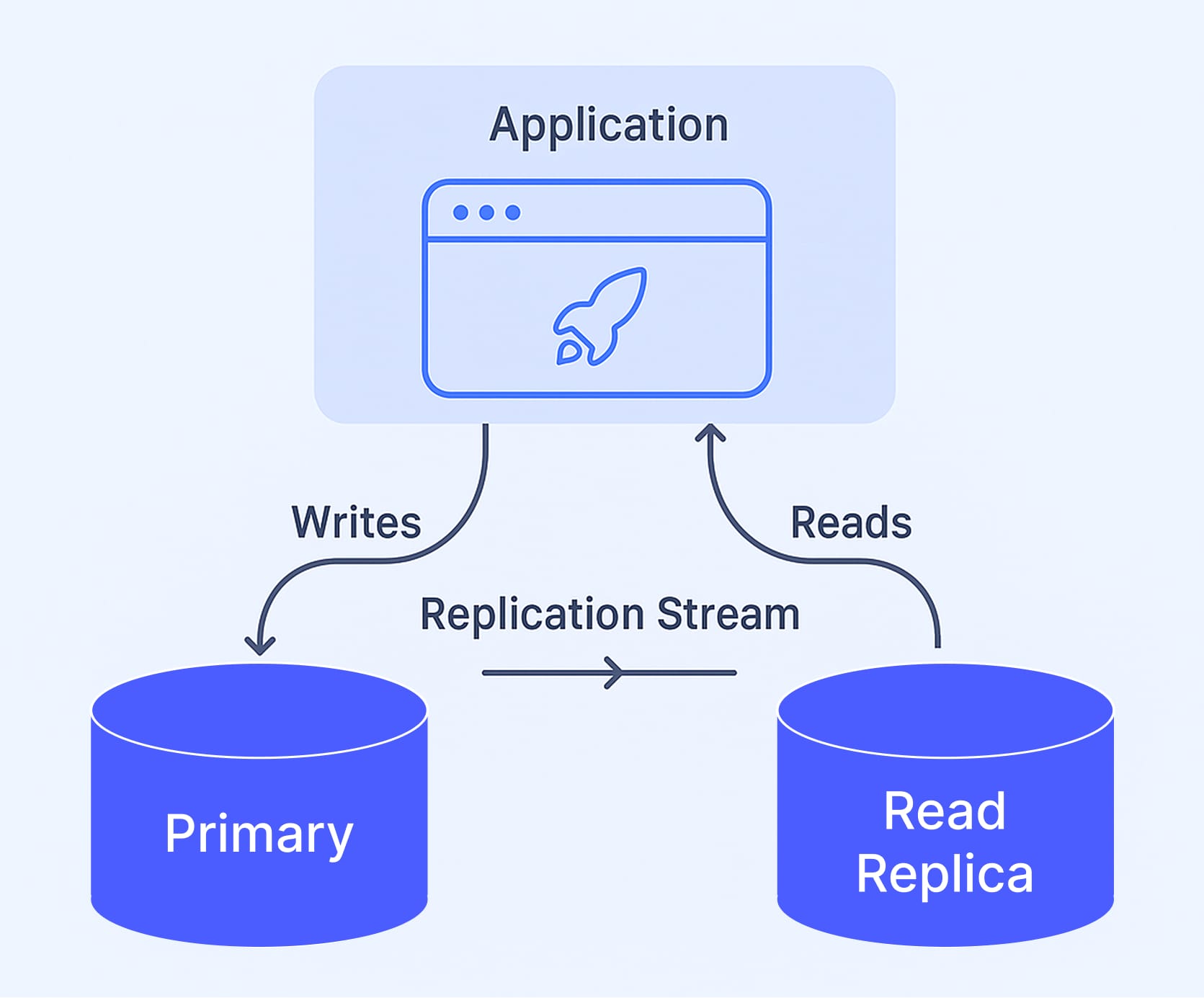
Routing all dashboard queries to the read replica worked surprisingly well, with the primary database seeing a 15% CPU reduction and dashboard p99 latency improving by 30%.
Since read replicas maintain exact copies of the primary, any index the team needed to add for dashboard charts still had to exist on the primary. This meant write performance on the primary was still degraded. There were still improvements to make since the dashboard could still take a few seconds to load.
Materialized Views
The team next needed a way to pre-compute dashboard query results:
CREATE MATERIALIZED VIEW monthly_regional_metrics AS
SELECT
  date_trunc('month', purchase_date) as month,
  customer_region,
  AVG(customer_age) as avg_age,
  SUM(purchase_amount) as total_revenue,
  COUNT(DISTINCT customer_id) as unique_customers
FROM purchases
JOIN customers ON purchases.customer_id = customers.id
GROUP BY date_trunc('month', purchase_date), customer_region;
Materialized views pre-compute and store query results, turning slow queries into simple table lookups. This successfully made the dashboard p99 latency drop 50%, but introduced the new challenge of the operational complexity of maintaining fresh views as data scale grew.
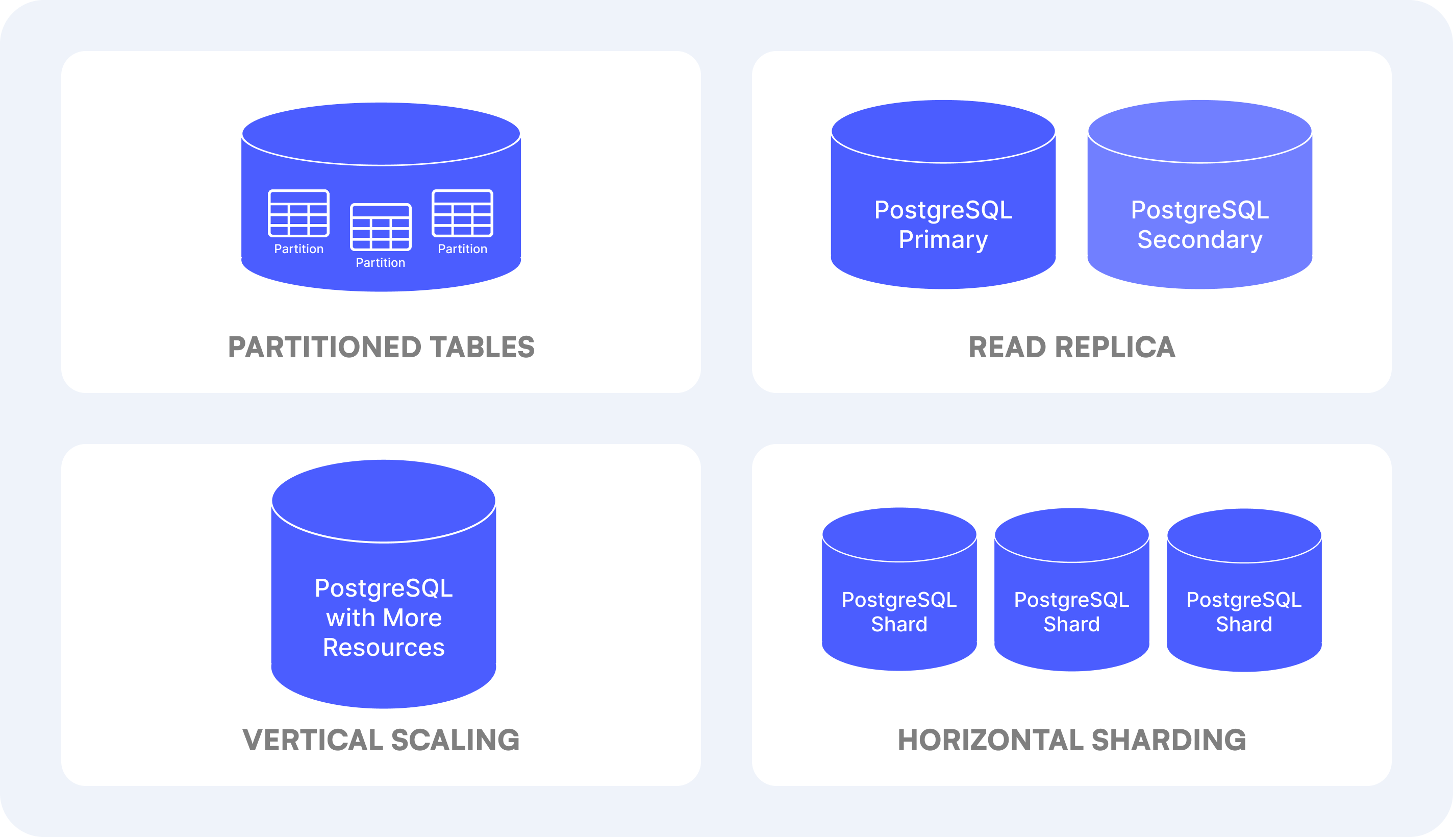
Table Partitioning
The team didn’t actually partition data, but I’ll list it here to be thorough:
CREATE TABLE purchases (
  id SERIAL,
  customer_id INTEGER,
  purchase_date TIMESTAMP,
  purchase_amount DECIMAL(10,2)
) PARTITION BY RANGE (purchase_date);

CREATE TABLE purchases_2019_q1 PARTITION OF purchases
  FOR VALUES FROM ('2019-01-01') TO ('2019-04-01');

CREATE TABLE purchases_2019_q2 PARTITION OF purchases
  FOR VALUES FROM ('2019-04-01') TO ('2019-07-01');
Partitioning divides large tables into smaller physical chunks. When a query specifies a date range, the database can scan only relevant partitions instead of the entire table.
Server Scaling
As our data volume continued to grow, the team considered a few other scaling approaches:
Vertical Scaling: The most straightforward of which is upgrading the hardware and giving it more resources. This continues to buy some time.
Horizontal Scaling: The most complex approach is distributing data across multiple servers called shards. This means implementing application-level logic to determine which shard to access when reading or writing data.
The approaches that were tried helped temporarily but didn't address the fundamental architectural issue, and the mismatch was becoming more apparent as the company scaled.
The Architectural Mismatch
Transactional databases such as PostgreSQL excel at:
- Quick point lookups and small range scans
- High concurrency for many small operations
- Strong data consistency guarantees
Analytical workloads like a dashboard have fundamentally different characteristics:
- They scan across table columns rather than accessing specific records
- They aggregate data across millions of rows
- They often need to access only a few columns from wide tables
When our dashboard query needed just purchase_date and purchase_amount from a 20-column table with say a million rows, PostgreSQL still reads all 20 million values. This massive I/O inefficiency is why our CPU and disk metrics kept hitting the ceiling.
That’s why databases made for analytical workloads store data in columnar format.
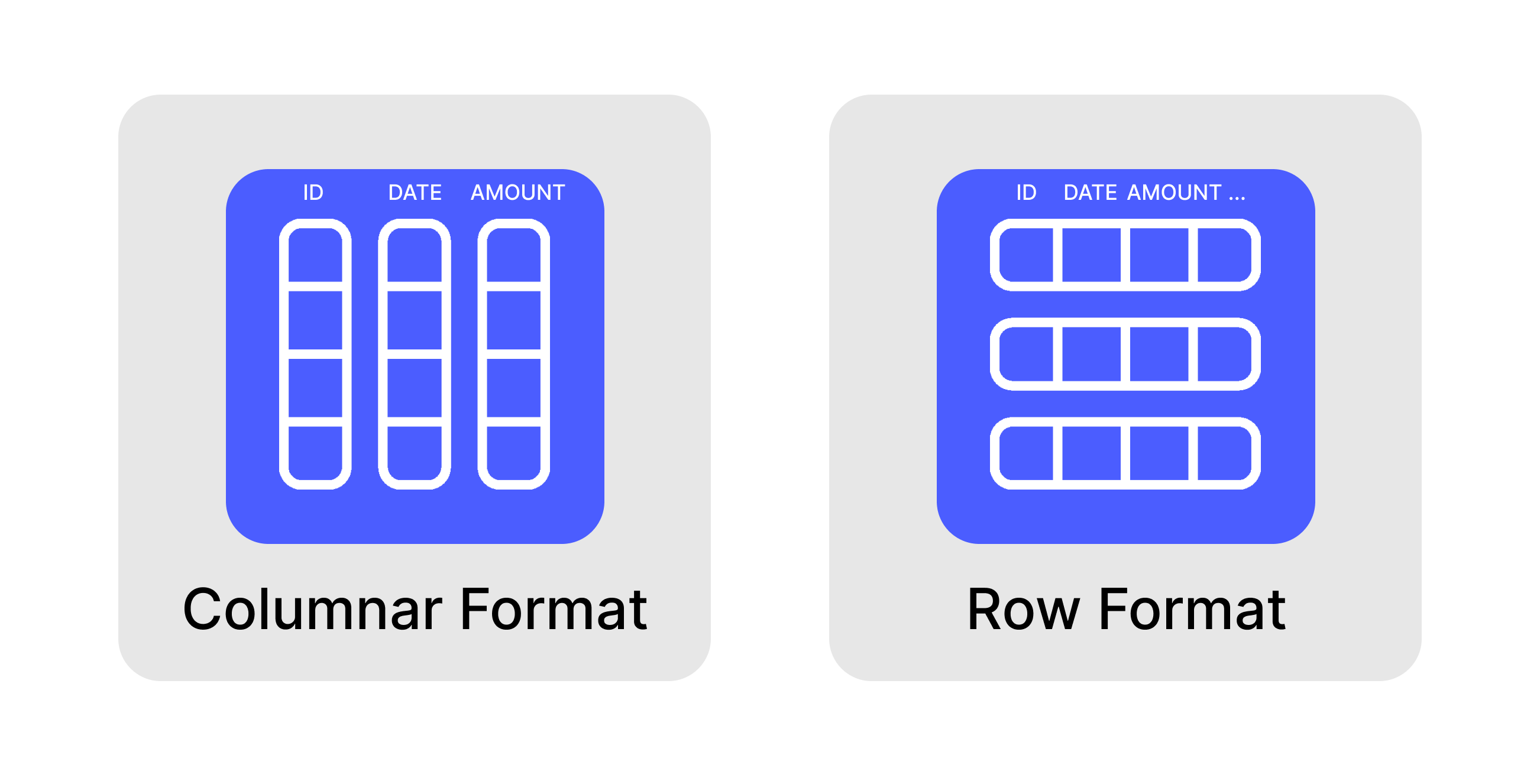
This columnar storage provides massive benefits for analytical queries:
- Only needed columns are pulled from disk
- Similar data in columns compresses better
- Operations can process batches of the same data type simultaneously
- Filtering happens before data is loaded into memory
Eventually, the temporary dashboard scaling workarounds weren’t enough and the team needed to move to an analytics optimized architecture.
The Data Warehouse
Before all scaling options were fully exhausted, the company had invested in setting up Snowflake with proper data pipelines, and all product teams were encouraged to leverage this new analytics infrastructure.
With the help from the data engineering team, they implemented a traditional extract-transform-load (ETL) architecture:
- Extraction: Airflow DAGs would run scheduled jobs that pulled data from our production PostgreSQL database
- Transformation: The extracted data underwent transformation steps before loading - cleaning values, applying business rules, and restructuring data.
- Loading: Finally, the transformed data was loaded into Snowflake tables optimized for analytical workloads.
For the dashboard to display this processed data, the team implemented a reverse ETL process that completed a data round-trip: production DB → Snowflake → back to production DB, but now with pre-computed aggregations ready for fast querying. This dropped dashboard load times to milliseconds!
The Batch Reality vs. Real-Time Promise
The team initially accepted a 24-hour refresh cycle for the dashboard metrics, comfortable with this temporary limitation based on the data team's roadmap promising real-time capabilities "soon." Our dashboard would clearly display: "Data updated daily at 4:00 AM UTC."
The company's leadership was understanding about this refresh cycle during the transition, but customers accustomed to seeing their latest transactions reflected immediately were confused by the sudden shift to day-old data. This created an unexpected support burden.
Unexpected Complexities
What started as a simple architectural improvement quickly revealed hidden operational costs:
Pipeline fragility: Weekly pipeline failures would result in cryptic error messages that the product engineering team struggled to troubleshoot, often requiring escalation to the busy data engineering team.
Dependency challenges: The promised real-time capabilities kept getting delayed as the data team discovered the true complexity of implementing Change Data Capture and Kafka streaming infrastructure.
While this architecture was theoretically correct, the company underestimated the operational overhead. Our mid-sized startup didn't actually have the petabyte-scale data that would justify the complexity, and our engineering team lacked a lot of data engineering talent. The organizational impact was equally problematic - our product team became dependent on an overextended data team, creating unclear ownership and delayed issue resolution.
For a company with a large data engineering org and massive data volumes, this architecture makes perfect sense. But for our relatively straightforward analytics needs, we had overcomplicated our infrastructure without considering the long-term operational and organizational costs.
Modern Analytical Solutions
Today, teams have simpler options available available. Several analytical databases can bridge the gap between transactional and analytical workloads without as much overhead as a Snowflake.
DuckDB: The Embedded Analytical Engine
DuckDB has emerged as a powerful columnar analytical database that can be embedded directly into applications - essentially SQLite for analytics:
- Embedded architecture: Runs inside a host process with bindings for languages like Python, with the ability to directly place data into structures like NumPy arrays
- Columnar-vectorized execution: Uses a columnar-vectorized query execution engine, where queries are still interpreted, but a large batch of values (a "vector") are processed in one operation
- Interoperability: Seamlessly works with the broader data science ecosystem
DuckDB is ideal for data scientists and analysts who need fast analytical capabilities integrated directly into their data workflows without the overhead of setting up a separate database server. It excels at scenarios like exploratory data analysis, ad-hoc queries, and processing moderately large datasets locally.
ClickHouse: High-Performance Analytical Database
Originally developed at Yandex for their analytics, Clickhouse now powers analytics at companies like Cloudflare and Uber. It's is a column-oriented DBMS built for analytical workloads at extreme scale:
- Distributed architecture: Designed to scale horizontally across clusters of commodity hardware
- Vectorized execution: Processes data in parallel using SIMD instructions for maximum performance
- Real-time ingestion: Can ingest large amounts of data with the Clickpipes integration
ClickHouse shines when dealing with massive datasets where query performance is critical.
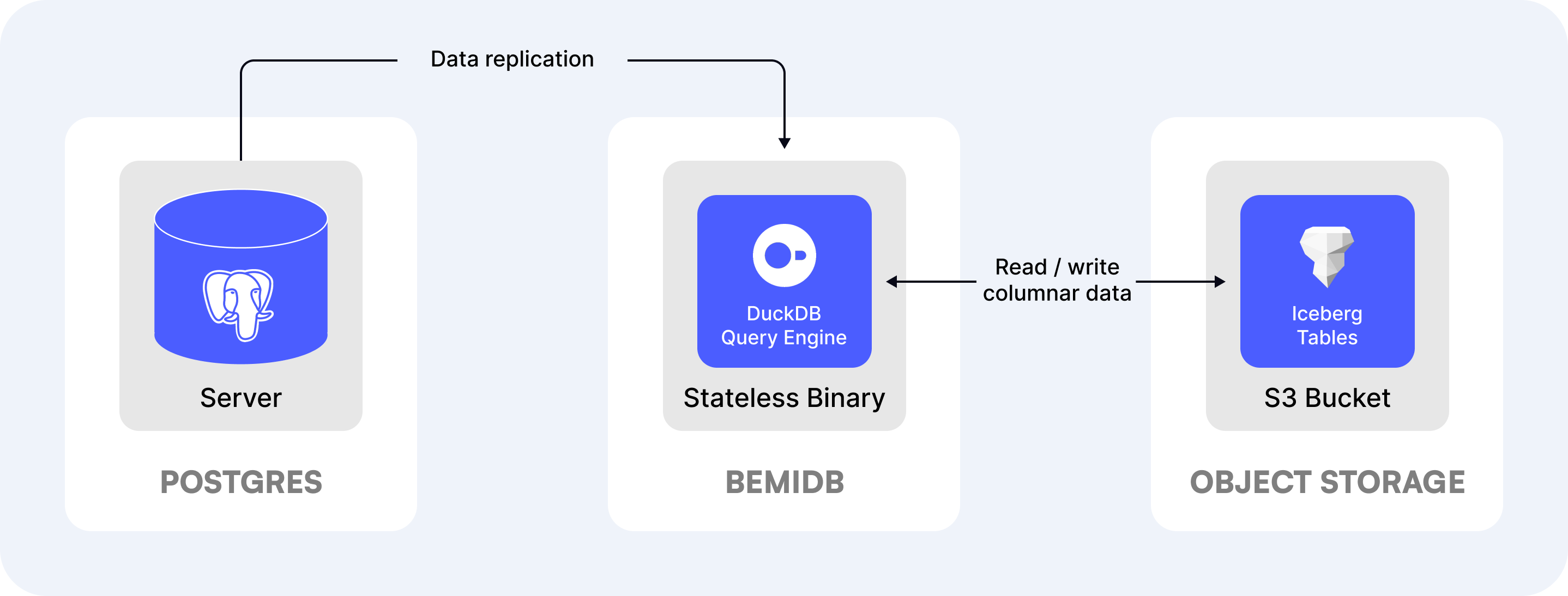
BemiDB: The Analytical Read Replica
Disclaimer: I’m a BemiDB open source contributor.
BemiDB is a single-binary PostgreSQL read replica for analytics:
- Automatic replication: Data syncs from Postgres with no pipeline code
- Open columnar format: Stores data either on a local file system or on S3-compatible object storage
- Full Postgres compatibility: Uses the same SQL syntax as PostgreSQL
BemiDB is ideal for teams trying to scale for analytics while staying close to PostgreSQL. The use cases it shines would be in-app analytics, BI queries, and centralizing PostgreSQL data.
Materialize: Streaming SQL for Real-Time Analytics
Materialize takes a different approach by focusing on real-time analytics using a streaming architecture:
- Incremental view maintenance: Updates query results as data changes
- Streaming architecture: Processes data changes in real-time as they occur
- Differential dataflow: Uses sophisticated algorithms to minimize computation
Materialize shines for use cases requiring real-time analytics on constantly changing data, including fraud detection, real-time notifications, and operational dashboards.
Choosing the Right Solution for Your Needs
The best choice would depend on your specific needs:
| Solution | Best For | Key Advantage |
|---|---|---|
| DuckDB | Embedded analytics, local analysis | Lightweight, no server needed |
| ClickHouse | Massive scale analytics | Extreme query performance |
| BemiDB | Simplicity, Postgres compatibility | Single binary, direct Postgres replication |
| Materialize | Real-time streaming analytics | Incremental view maintenance |
A Simpler Path Forward
Instead of the painful progression most companies follow:
- Query production directly until it breaks
- Add indexes until writes become slow
- Build complex ETL pipelines to data warehouses
- Create reverse ETL to bring data back to the application
Consider this simpler approach:
- Keep transactional workloads on your production database
- Use a columnar analytical engine for reports and dashboards
- Only move to a full data warehouse when you truly need to integrate many different data sources or process petabytes of data
This approach would’ve saved that team months of trouble. The mid-sized startup needed operational simplicity and the team first and foremost wanted to eliminate late-night pages, pipeline debugging, and the performance dance of trying to make the transactional database not meltdown. The right solution for you will depend on your specific requirements around data volume, real-time needs, and data org maturity.
There are several open-source solutions mentioned worth exploring, including DuckDB, ClickHouse, BemiDB, and Materialize. Each has different trade-offs that might make it the right fit for your specific needs.